
Top 10 Snowflake Query Optimization Tactics
Updated 5-May-2023. (Completely Rewritten)

Top 10 Tips for Snowflake Query Optimization
The Snowflake query optimizer implements many advanced query-tuning techniques. However, Snowflake Indexes are not supported on default tables, raising an important question: How on Earth can you tune SQL queries on a database without indexes?
This article explains precisely how, with a list of the top 10 Snowflake optimization tips.
If you're already an expert on Snowflake, feel free to skip to the summary and conclusion listing query optimization techniques.
Why Does Snowflake Performance Tuning Matter?
One of the most significant differences between Snowflake and on-premises databases like Oracle or SQL Server is that query optimization in Snowflake will deliver faster results AND save money. I'm so confident I think there's a potential role for system tuning experts whose job is to help maximize performance and reduce costs.
Unlike on-premises databases, where you purchase the hardware and licenses up front, Snowflake charges you per second while the compute resources (a Virtual Warehouse) are active.
For successful performance tuning in Snowflake, you, therefore, need to decide on a priority:
Reduce query elapsed times: A frequent priority for end-user queries, this can also be vital for fast data ingestion and transformation to deliver data quickly for analysis. This is the main focus of this article.
Reduce Cost: If the priority is to reduce Snowflake cost rather than maximize query performance, the article on Snowflake cost management may be more helpful. However, both articles work together to deliver the same end goal: faster queries for less spending.
In summary, Snowflake query tuning prioritizes tuning SQL statements, whereas Snowflake cost control needs a more strategic approach, paying attention to virtual warehouse size and deployment.
The Snowflake Architecture Explained
Before diving into specific Snowflake SQL tuning techniques, the architecture illustrated in the diagram is worth considering.
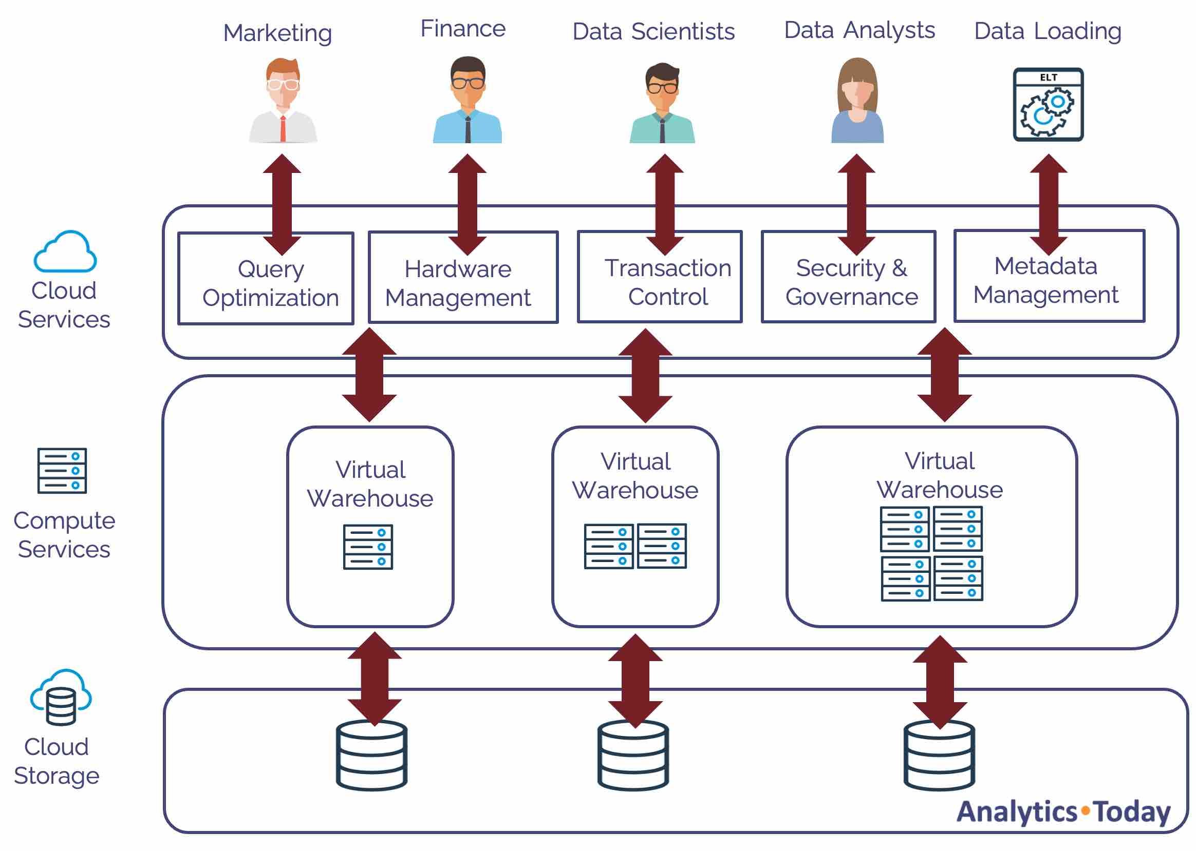
Snowflake is not just a single machine but three interconnected computer systems, each with its own auto-scaling hardware and software.
The diagram above illustrates the layers, including:
The Cloud Services Layer: This accepts the connection, and the Snowflake query optimizer tunes the query, potentially re-writing the code to maximize SQL query performance.
The Compute Services Layer: Executes the query on a Virtual Warehouse, a cluster of machines ranging from 1 to 512 times the compute processing. Each node in the cluster is a computer with eight CPUs, memory, and Solid State Disk (SSD) for temporary storage. Virtual warehouse storage, which is considerably faster than disk storage, is called local storage.
The Cloud Storage Layer: Physically stores the data in blob storage. Typically held on a hard disk, Cloud Storage is called Remote Storage in Snowflake.
Snowflake Caching
One of the techniques Snowflake uses to maximize Snowflake query performance involves caching results in both the Virtual Warehouse and Cloud Services layer. The diagram below illustrates how Snowflake caches data.
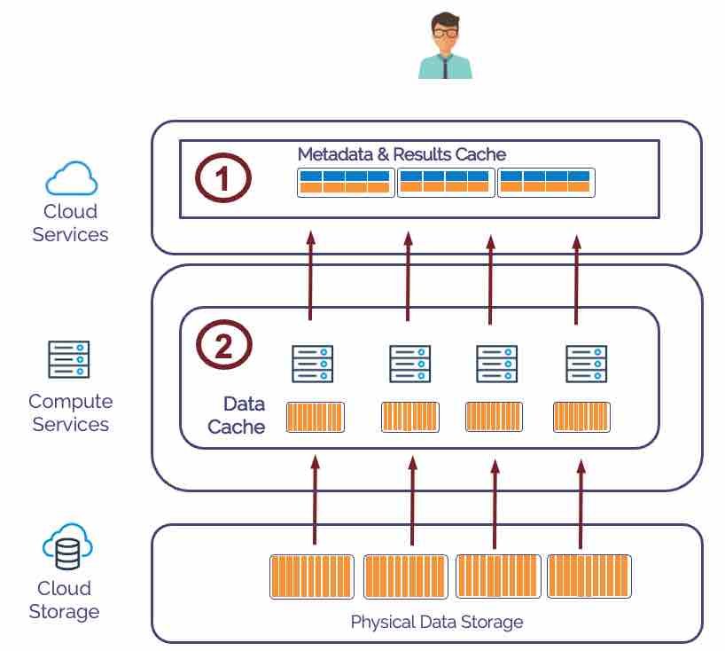
In summary, Snowflake maintains a cache at the following layers:
Cloud Services: This holds the Metadata and Results Cache. The Metadata Cache maintains the count of rows, and distinct and null values, while the Results Cache contains the result set of every query executed during the past 24 hours.
Virtual Warehouses: Use a Least Recently Used (LRU) algorithm to cache raw data in fast SSD. Snowflake can execute queries against data held locally using the Data Cache, avoiding slower remote storage access.
Typically, SQL queries handled by the Metadata or Results cache return within milliseconds and don't even need a Virtual Warehouse. Queries run against the Data Cache can improve query performance by as much as sixteen times. You can read more in the article on Snowflake Caching.
How does Snowflake Execute Queries?
Understanding how queries are executed on each node is essential to Snowflake query tuning. The diagram below shows how the Snowflake query optimizer uses metadata to track the location of every micro-partition on the remote storage.
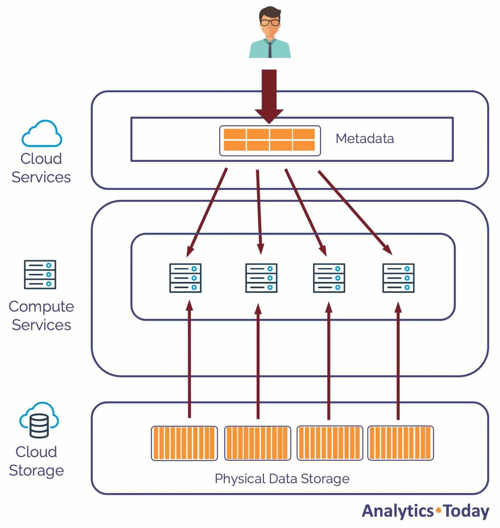
The diagram above illustrates how the Snowflake query optimizer uses the metadata to eliminate partitions and reduce the number of micro-partitions that need to be fetched. The metadata is distributed across the nodes in the Virtual Warehouse, which executes the query in parallel against the relevant data sub-set. The results are calculated in parallel before being returned to the user via the Results Cache.
This leads to one of the most important insights about Snowflake: increasing the warehouse size doesn't increase the speed but maximizes throughput as the workload is distributed across more nodes.
It is, however, essential to distinguish between (in this example) running queries on a MEDIUM-size warehouse with four nodes and running queries on a multi-cluster warehouse – for example, an XSMALL warehouse scaled out to provide four clusters. Unlike a MEDIUM size warehouse, where the query is executed in parallel across all nodes, a scale-out deployment distributes the concurrent queries across the available clusters.
Using the first approach, the query is executed in parallel using all four nodes. The second approach runs the query on just one server but supports more concurrent queries.
Query Tuning by Zone
Web-scale data warehouse systems are often remarkably complex, and it's sensible to approach the query tuning task systematically by subject areas or zones. The diagram below illustrates the zones of a typical Data Warehouse, and each needs a slightly different approach.
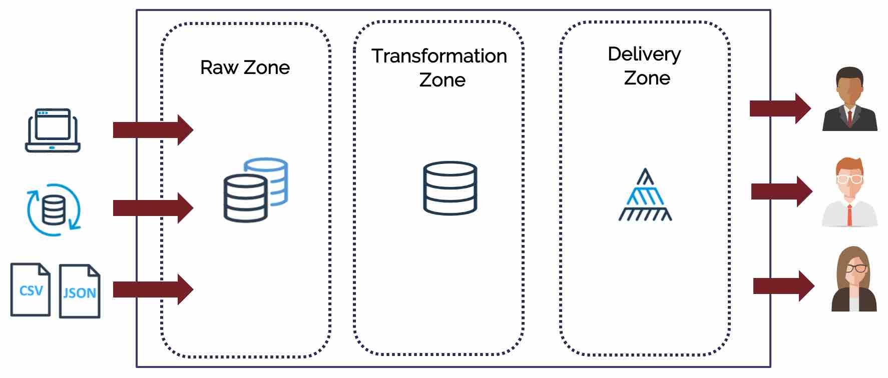
The above diagram shows how data is loaded from source systems into the Raw Zone, which is then integrated and transformed in the Transformation Zone before being restructured (probably using Dimensional Design) for analysis and consumption in the Delivery Zone.
Data processing in the Raw Zone primarily involves data loading, which will be covered in a separate article. At the same time, the Transformation Zone focuses on maximizing throughput – integrating and aggregating data as quickly and efficiently as possible. Finally, queries in the Delivery Zone deliver results to end-users and prioritize minimizing latency – the delay between submitting a query and providing results.
Regardless of the overall data architecture used, whether it is the Kimball, Innmon methodology or Data Vault, the overall approach remains the same, and Snowflake works well regardless of data warehouse design methodology.
Either way, each of these zones needs a slightly different tuning approach. This article will describe Snowflake query tuning tactics for the Transformation and Delivery areas.
Maximizing Transformation Throughput
Increasing warehouse size is one of the simplest and most effective ways of improving transformation performance. However, as indicated in an article on Snowflake Cost Management, while it is possible to reduce query elapsed time from four hours to just 60 seconds, scaling up is only cost-effective if the query executes twice as fast.
The diagram below illustrates another technique for maximizing transformation speed: utilizing Snowflake's power to execute tasks in parallel and scale out to maximize concurrency and deliver almost unlimited throughput.
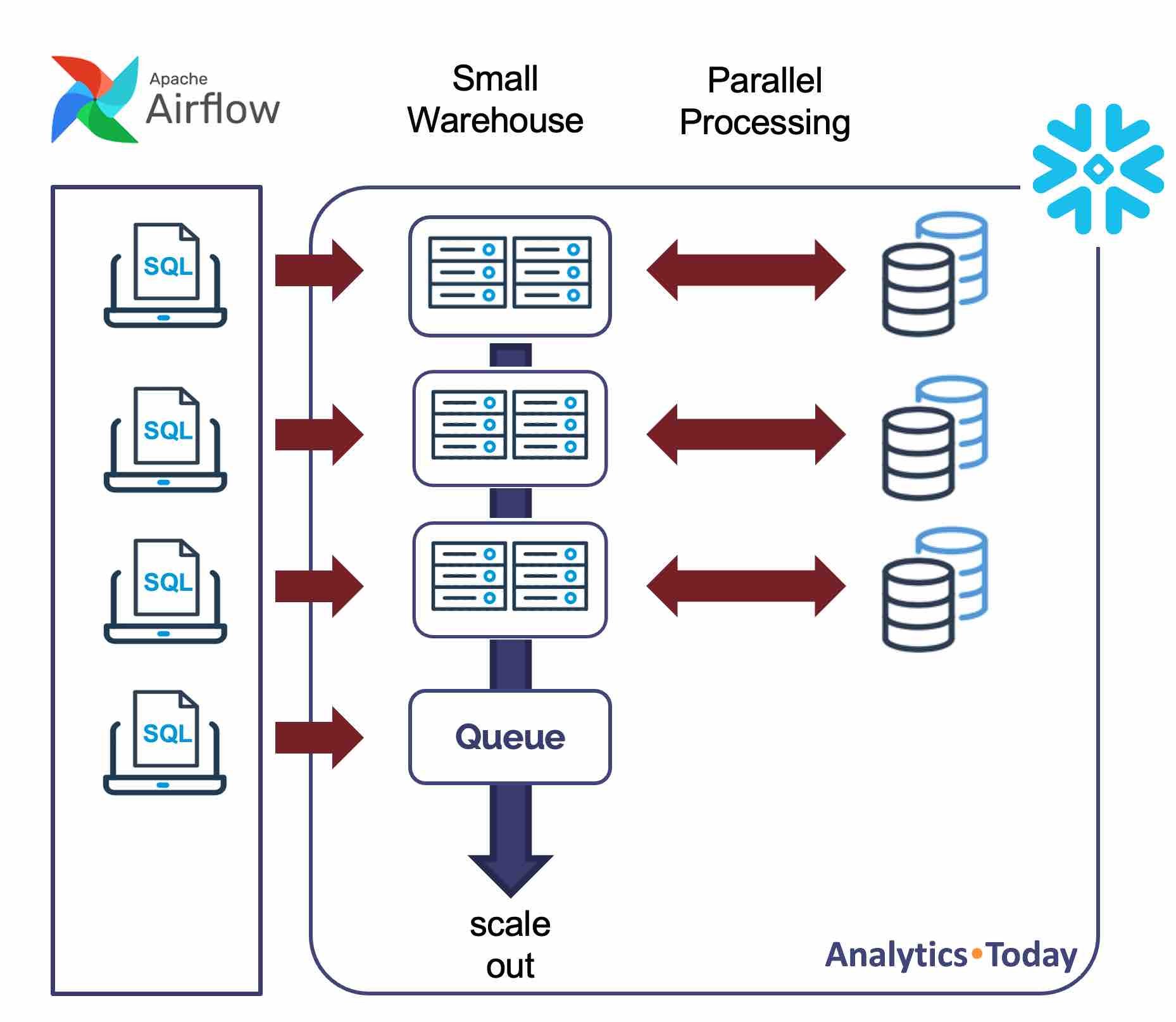
Unlike on-premises database systems, whereby increasing the system workload tends to negatively impact elapsed times for all users, Snowflake has built-in workload management. As queries are submitted, and the Virtual Warehouse approaches full capacity, subsequent queries are suspended on a queue until resources are available.
The SQL statement below configures the warehouse to automatically scale out to a maximum of three clusters which means it avoids query queuing by automatically allocating additional same-size clusters if queuing is detected.
alter warehouse prod_transform_standard_wh set
   min_cluster_count = 1
   max_cluster_count = 3
   scaling_policy = ‘ECONOMY’
   auto_suspend = 60;
Using this technique, a single transformation warehouse can process several tasks in parallel, provided each job is executed in a new session.
Using the SCALING_POLICY of ECONOMY, the warehouse waits until it detects six minutes of work is queued before starting another cluster which prioritizes throughput while controlling spending. This approach is sensible for transformation workloads where individual query latency is not the main priority.
Avoid Row-by-Row Processing
Sometimes it is more important to understand what to avoid; row-by-row processing is a classic example. Take the following SQL statement that copies a million entries from the CUSTOMER table in the database SNOWFLAKE_SAMPLE_DATA.
insert into customer
select *
from snowflake_sample_data.tpcds_sf100tcl.customer
limit 1000000;
Using an X-Small warehouse, this completes in around five seconds execution time, whereas the following SQL copies just ten rows in a loop using Snowflake Scripting:
declare
v_counter number;
begin
  for v_counter in 1 to 10, do
     insert into customer
     select *
     from snowflake_sample_data.tpcds_sf100tcl.customer
     limit 1;
  end for;
end;
The above script takes 11 seconds to insert just ten rows in a loop, whereas a single SQL statement can copy a million rows in half the time. This demonstrates the bulk processing power of a single SQL statement can deliver around a million times the throughput of row-by-row processing.
The following query can be used to help identify row-by-row processing on the Account:
select query_text, session_id, user_name, count(*)
from query_history
where warehouse_size is not null
and   query_type in ('INSERT', 'UPDATE', 'DELETE', 'MERGE')
and   rows_produced = 1
group by 1, 2, 3
having count(*) > 10
order by three desc;
The query above should be periodically executed to help detect queries repeatedly executed within the same session as these are a high priority for tuning.
Simplify Transformation Queries
One common design pattern frequently seen on migrations from Teradata to Snowflake involves building an entire ELT pipeline in a single SQL statement which makes it challenging for the Snowflake query optimizer to tune.
The SQL statement and diagram below illustrate a common scenario:
insert into sales_history
select *
from sales_today;
While the above query appears to be simple, in reality, SALES_TODAY is implemented as a complex view that, in turn, builds upon sedimentary layers of increasingly complex views, which quickly becomes unmanageable to understand and even more challenging to modify.

This approach becomes problematic because one of the most critical Snowflake optimization techniques relies upon Snowflake's ability to estimate the cardinality of every JOIN operation. This presents no issue for the lower-level joins where Snowflake can directly access table statistics. However, this becomes an increasing challenge when the data has been summarized and grouped at multiple levels.
For example, if Snowflake needs to join two tables, it uses a Hash Join algorithm to load the smaller table into memory and scan the larger table from remote storage. Suppose the query has several layers of JOIN and GROUP BY operations. In that case, this becomes increasingly difficult and sometimes leads to a poor query plan whereby Snowflake attempts to read the larger table in memory.
The screenshot below shows an example of a complex Query Profile, which involves a considerable number of joins which should ideally be avoided as it both risks poor query performance and makes the query challenging to understand.
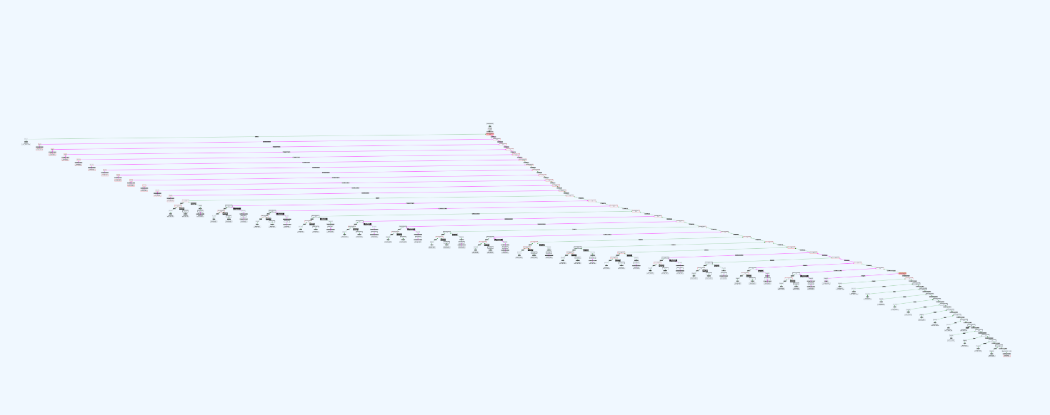
Amazingly Complex Snowflake Query Profile
The diagram below illustrates a potential solution to the problem. Instead of executing the statement as a single query, break the problem down into multiple queries that write results to transient tables.
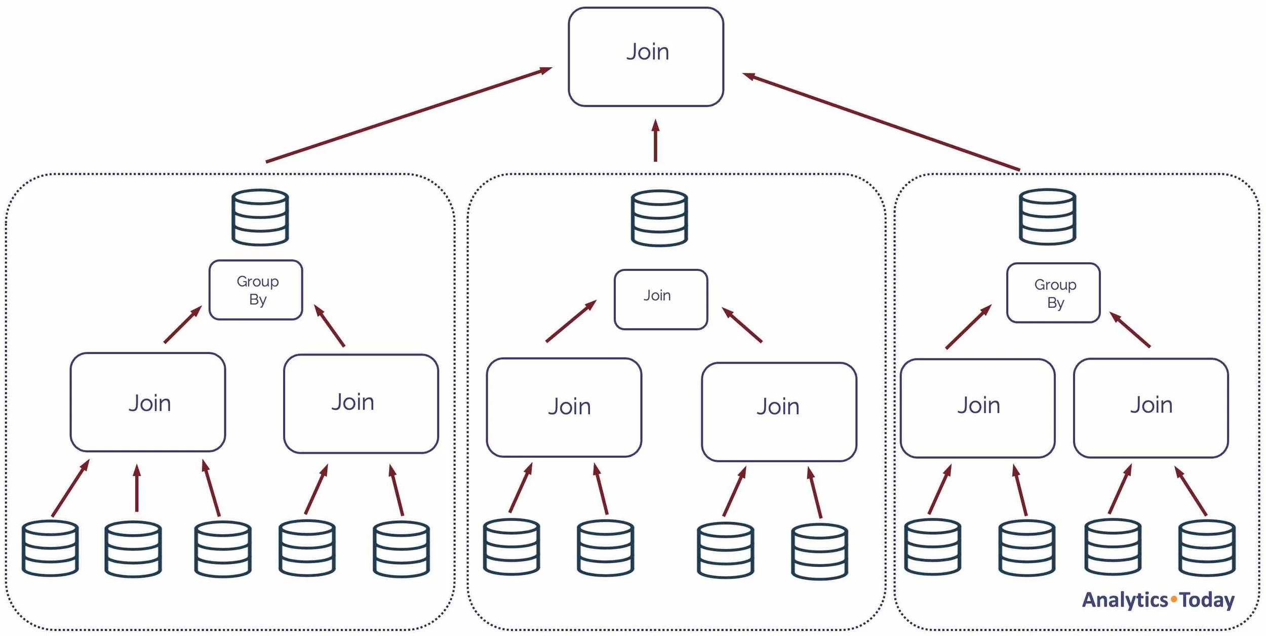
Simple Design to Break Down a Complex Snowflake Query
This approach can be implemented in several ways, including a series of parallel executing transformation jobs to build the intermediate tables or using Dynamic Tables.
In addition to the potential performance gains of breaking down the problem and executing components in parallel, the solution is easier to understand. It also leads to query plan stability for each query component.
Avoid Snowflake Spilling to Storage
The diagram below illustrates the internal structure of an X-Small Virtual Warehouse, which consists of CPUs, memory, and local storage (SSD). Snowflake always tries to execute sort operations in memory to maximize query performance. Still, if the sort is too large, it will need to spill intermediate results to slower local storage and potentially even slower remote storage.
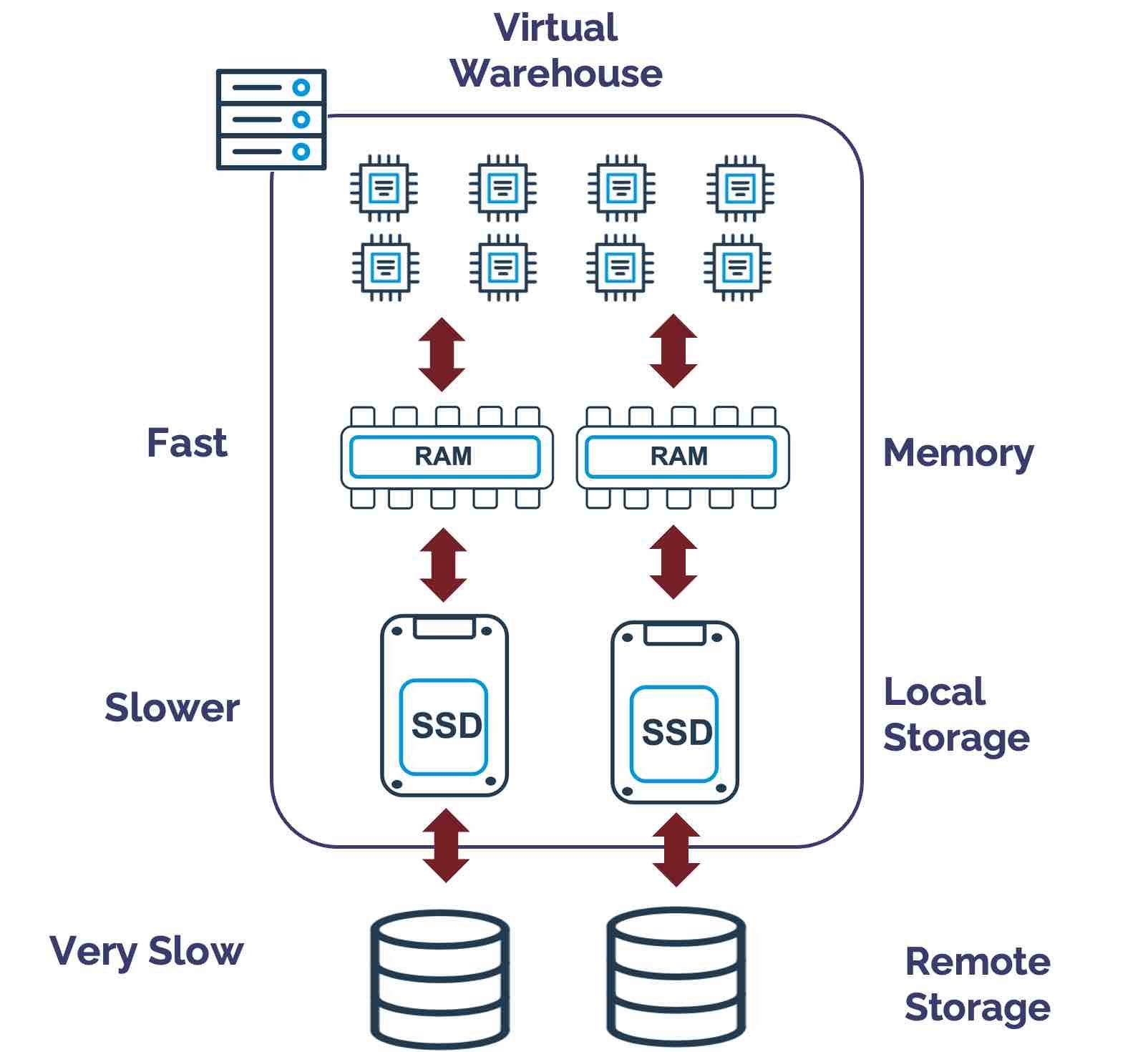
Analytic (window) functions produce sort operations, along with GROUP BY, ORDER BY, and JOIN operations, where both tables are enormous.
Spilling to storage impacts query performance because memory is faster than an SSD, which is much quicker than a remote disk. In addition to impacting query performance, this increases cost as queries take longer to run, preventing virtual warehouses from suspending.
The most effective solution to avoid spilling is to execute the workload on a larger Virtual Warehouse. Each T-shirt size distributes the load across more nodes, and each node has memory and SSD, which makes scaling up the most effective method of reducing spilling. In extreme cases, increasing the warehouse size may reduce the overall cost.
The query below will quickly identify each warehouse's spilling number and extent to storage. As this is based upon query-level statistics, it is possible to drill down to identify specific SQL.
select warehouse_name
,      warehouse_size
,      round(avg(total_elapsed_time)/1000) as elapsed_seconds
,      round(avg(execution_time)/1000) as execution_seconds
,      count(iff(bytes_spilled_to_local_storage/1024/1024/1024 > 1,1,null)) as count_spilled_queries
,      round(sum(bytes_spilled_to_local_storage/1024/1024/1024))  as local_gb
,      round(sum(bytes_spilled_to_remote_storage/1024/1024/1024)) as remote_gb
from Snowflake.account_usage.query_history
where warehouse_size is not null
group by 1, 2
having local_gb > 1
order by six desc;
Maximize Snowflake Pruning
As data is loaded, Snowflake organizes data into 16MB variable length chunks called micro-partitions. It automatically captures metadata statistics about every entry, including every column's minimum and maximum value. The diagram below illustrates a potential data layout assuming data is loaded at the end of each month.
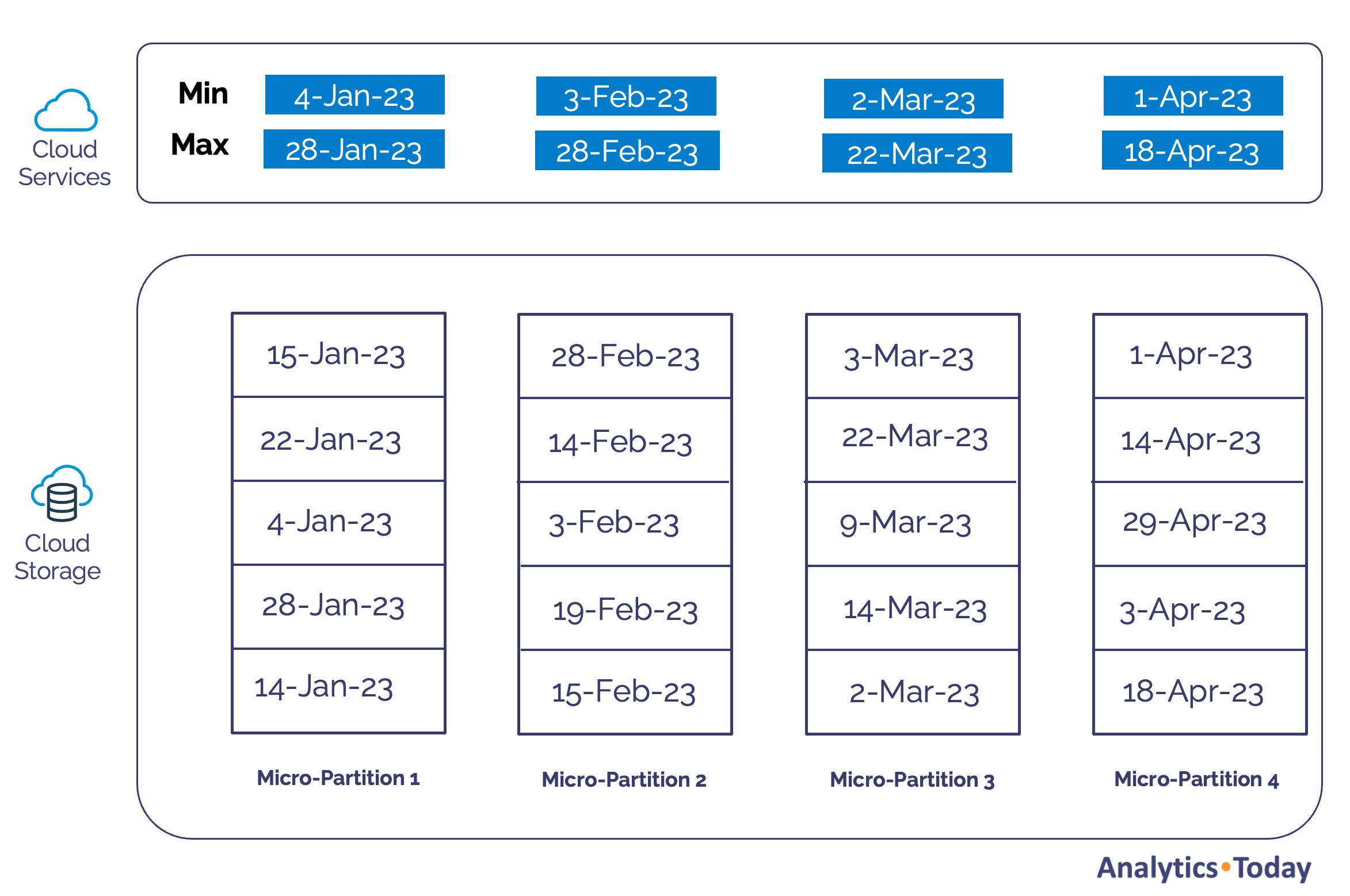
Snowflake Partition Pruning Example
The diagram above shows that as data is loaded each time, it's loaded into one or more micro-partitions in Cloud Storage. At the same time, the Cloud Services layer captures the metadata statistics for each column.
Snowflake uses the metadata to apply partition pruning automatically. For example, if the following query was executed, the optimizer narrows the search to micro-partitions 2 and 3, ignoring all other micro-partitions.
select *
from sales
where sale_date between ’01-Feb-23’ and 31-Mar-23’;
On a large table with thousands of micro-partitions, this Snowflake Clustering technique can have a massive impact on query performance, particularly when the clustering is maintained using a Cluster Key.
Cluster Keys are best deployed in the Delivery Zone as frequent updates tend to disrupt the clustering, which can lead to increased credit spend as tables are re-sorted by the background Automatic Clustering Service.
The following query can identify SQL statements that scan huge tables and fetch at least 80% of the rows and are, therefore, a potential candidate for improvement.
select query_type
,      warehouse_size
,      warehouse_name
,      partitions_scanned
,      partitions_total
,      partitions_scanned / nullifzero(partitions_total) * 100 as pct_scanned
from sb_query_history
where warehouse_size is not null
and   partitions_scanned > 1000
and   pct_scanned > 0.8
order by partitions_scanned desc,
         pct_scanned desc;
Optimize the WHERE Clause
Partition pruning relies upon the WHERE clause filtering out data, but several simple mistakes can inadvertently reduce partition pruning leading to long execution time. For example, consider the query below, which starts with a wild card and therefore has no partition pruning:
select *
from sales
where customer_name like ‘%RYAN’;
Likewise, the following query wraps the column in a User Defined Function (UDF), which makes it almost impossible for Snowflake to apply partition elimination:
select *
from sales
where profit_calculation(sale_value) > 100;
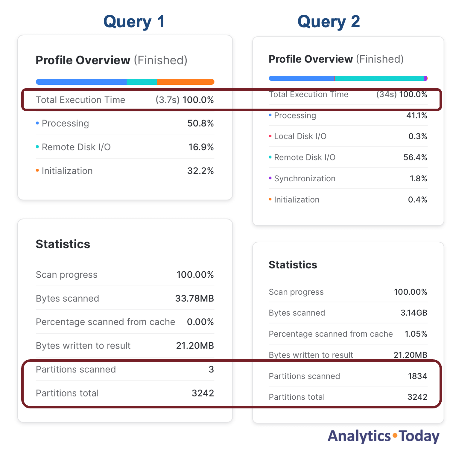
Similarly, wrapping columns in the WHERE clause can also significantly reduce partition elimination, leading to poor query performance. Take the following two queries, which produce the same results:
-- Query 1:

select *
from SNOWFLAKE_SAMPLE_DATA.TPCH_SF1000.ORDERS
where o_orderdate = to_date('01-04-92','DD-MM-YY');

-- Query 2:

select *
from SNOWFLAKE_SAMPLE_DATA.TPCH_SF1000.ORDERS
where to_char(o_orderdate,'DD-MM-YY') = '01-04-92';
As the screenshot illustrates, query 1 prunes over 600 times more micro-partitions than query 1 and is almost ten times faster at 3.7 instead of 34 seconds execution time.
For this reason, you should (where possible) avoid wrapping WHERE clause columns in functions but try rewriting the condition to compare to a fixed value.
For the same reason, you must always store data in the native data type. For example, if data is provided as text but represents numeric or date values, you must define the columns as NUMBER or DATE to maximize partition elimination. This also significantly improves data compression, which minimizes disk I/O and helps improve query performance.
Maximize Query Concurrency
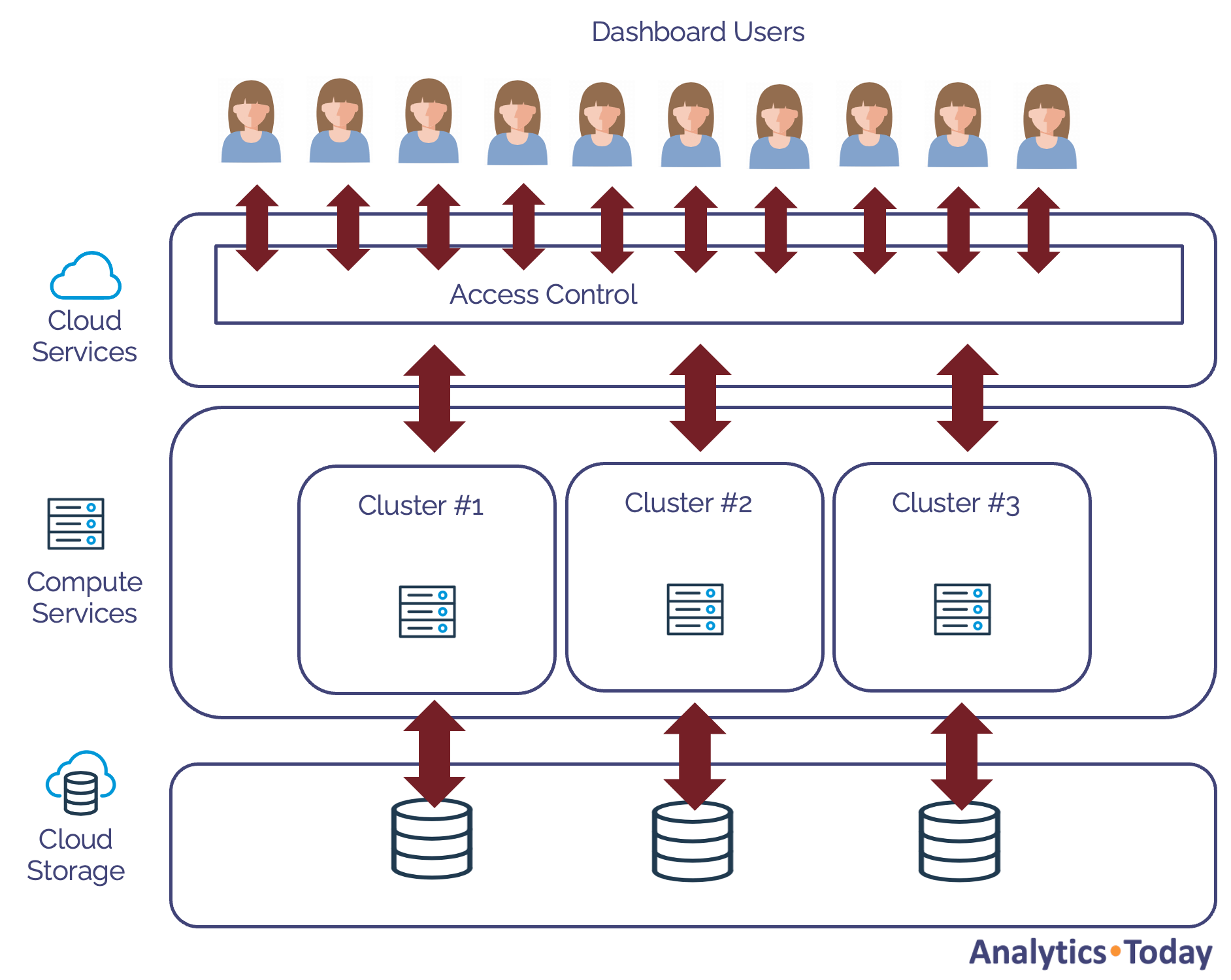
The same multi-cluster scale-out approach described above can support many end-user queries in the same warehouse. The diagram below illustrates how additional clusters are automatically started as concurrent queries increase.
As additional users submit queries, the scale-out approach distributes the workload across all available clusters instead of being executed across all available clusters. Unlike the scale-up approach, which increases throughput, this technique improves query concurrency.
Using this method, it is sensible to set the SCALING POLICY to STANDARD, which will start additional clusters immediately and avoid queries being queued waiting for resources. The SQL below shows the command used to list the average number of milliseconds of queries spent waiting for resources.
select warehouse_name                    as warehouse_name
,      warehouse_size                    as warehouse_size
,      round(avg(execution_time))        as avg_execution_time
,      round(avg(total_elapsed_time))    as avg_elapsed_time
,      round(avg(queued_overload_time))  as avg_overload_time
,      round(((avg_elapsed_time / avg_overload_time)* 100),1) as pct_overload
from Snowflake.account_usage.query_history
where warehouse_size is not null
group by 1,2
order by 2;
If the above query returns no rows, it may indicate that the warehouses are over-provisioned and not cost-efficient. However, when the queued overload time becomes a significant percentage of the overall elapsed time, this is a potential concern and should be addressed.
Use the Snowflake LIMIT rows or TOP clause
The simplest but most effective way of improving the performance of SELECT queries is to include a TOP or LIMIT clause. You often need to see the first few rows in a table to understand the contents, leading to a SELECT * FROM TABLE command.
As the SQL below shows, including a TOP or LIMIT clause avoids fetching the entire table into the Cloud Services Result Cache, and for huge tables, results can return in seconds rather than minutes.
However, the LIMIT or TOP clause also improves queries with an ORDER BY clause. For example, the first query below returns in just over two minutes on an X-SMALL warehouse, whereas the second query, which returns the top ten entries, is twelve times faster, taking just six seconds to complete.
-- 2m 5s
select *
from SNOWFLAKE_SAMPLE_DATA.TPCH_SF100.ORDERS
order by o_totalprice desc;

-- 6 seconds using SELECT TOP 10
select top 10 *
from SNOWFLAKE_SAMPLE_DATA.TPCH_SF100.ORDERS
order by o_totalprice desc;
Avoid SELECT *
Like most analytic database systems, including Vertica and Redshift, Snowflake stores data in column format. The diagram below illustrates the difference between Row Storage (on the left), optimized for OLTP systems, and Column Storage (on the right), which includes significant compression improvements and faster I/O.
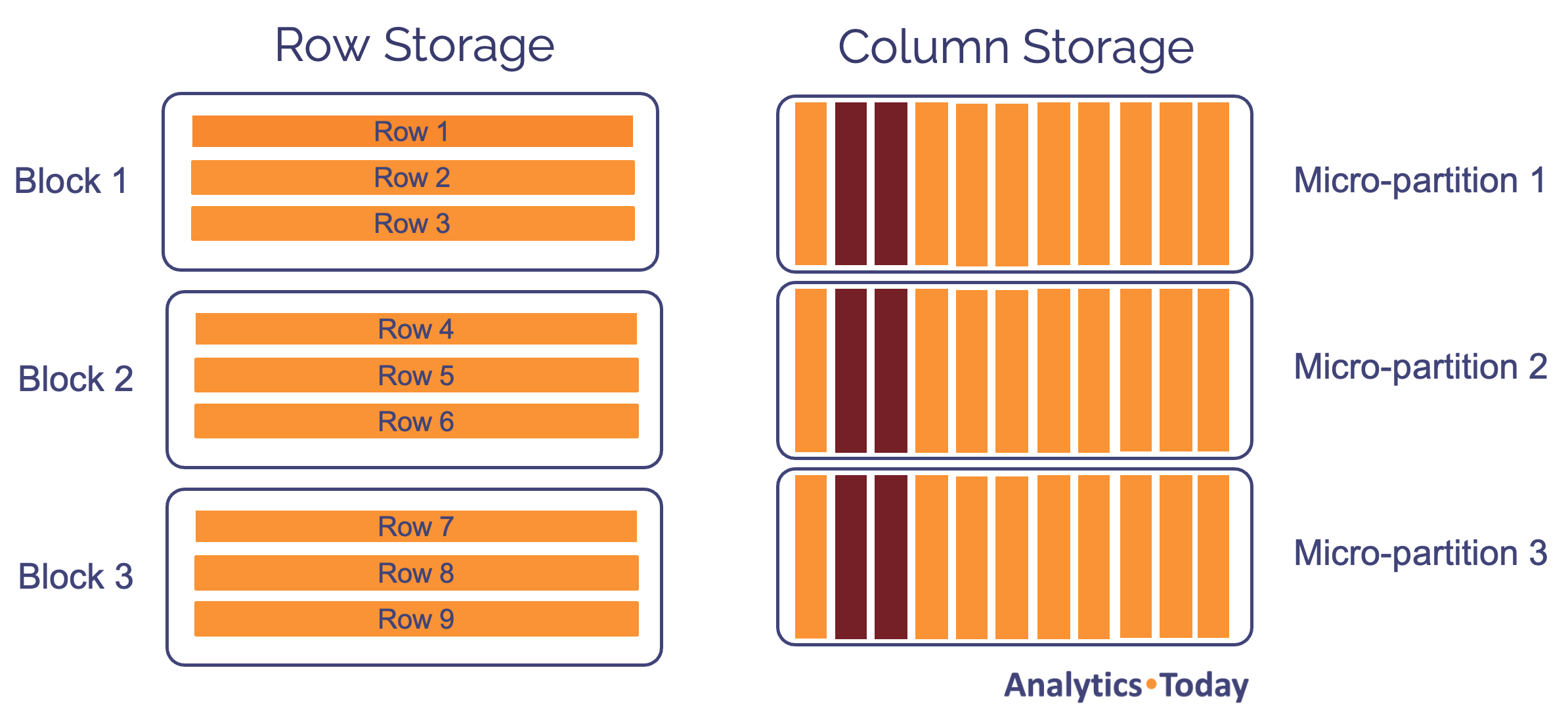
Professor Mike Stonebraker has indicated that columnar databases are around 100 times faster at analytic queries than row-oriented ones because they only read the column values needed to satisfy the query.
For example, if the following query were executed on a table with 100 columns, it would retrieve just 2% of the columns from disk storage.
select region, sum(sales)
from sales
group by region;
However, this leads to another of the Snowflake performance best practices – avoid SELECT * from tables and only retrieve the columns needed.
While this is not an issue for online queries, we need to avoid this in production systems as it has two essential benefits:
1. It reduces the data volume transferred from remote storage into memory.
2. It ensures efficient use of Virtual Warehouse Cache storage.
Both of these benefits help maximize overall query performance.
Consider Snowflake Performance Features
Snowflake provides several innovative tools to help maximize query performance. In each case, they target a specific SQL performance challenge. I’ve written a series of articles about each of these including:
Search Optimization Service: This can be used to find a small number of rows (typically less than 100) from a large table will millions or billions of rows.
Query Acceleration Service: This provides an automatic scale-up facility to help improve throughput and reduce latency.
Data Clustering: This can be used to improve partition elimination. This is especially useful on Fact Table queries in the Delivery Zone.
Materialized Views can aggregate or filter sub-sets of data while providing a guaranteed consistent view of the underlying data. (Article coming soon)
In Snowflake, Indexes are (mostly) Evil.
At the beginning of this article, we explained that Snowflake indexes are not supported on standard (default) tables, potentially making performance optimization challenging. This raises the obvious question – why not?
The short answer is that indexes destroy load performance. But first, we should consider the question: what is an Index?
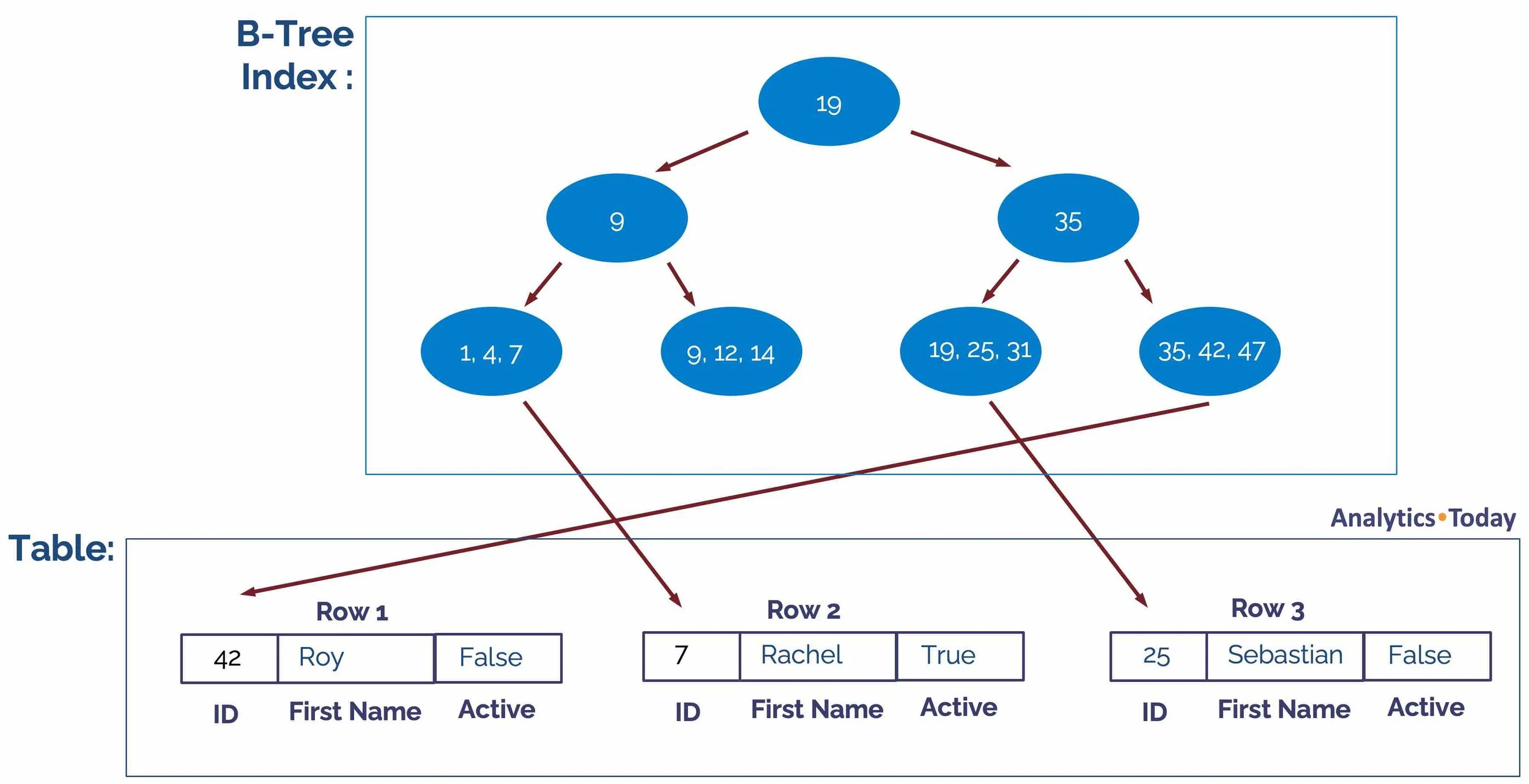
The diagram above illustrates a B-Tree index proposed by Bayer and McCreight in July 1970. The B-Tree index uses an in-memory structure to quickly narrow down the search for a given key, followed by a random-access lookup against disk storage. It works on the principle that in-memory access is about 100,000 times faster than disk storage, and most (if not all) of the index is often cached in memory.
For example, if you were looking to fetch the data for ID = 25, it's a simple three-step process:
Root Node: Is 25 > 19? Yes - fetch node 35.
Node: 35: Is 25 > 35? No - fetch node 19-31
Node 19-31: Includes a pointer to row 25 on the disk.
While B-Tree indexes are typically fast for single-row random access lookups, most data warehouse queries process thousands or even millions of rows and seldom look up a single row. Single-row processing is a therefore a significant anti-pattern on default tables. However, the main reason why Snowflake doesn't support indexes except on hybrid tables is the massive impact on load performance.
My benchmark tests demonstrate Snowflake can quickly load 36GB of data in around 40 seconds on an X2LARGE. A 5.2 GB/Min rate would be impossible with even a single index on the table.
But Snowflake Indexes are Supported
As indicated above, Snowflake indexes are not supported on default tables intended for OLAP queries that fetch and summarize millions of rows. However, indexes are supported on Unistore Hybrid Tables, which are designed for single-row operations.
Unlike default tables, Hybrid tables are designed to support analytic and transaction processing (OLTP) workloads. This new type of table will support:
Primary Key Constraints: Primary key constraints are mandatory and are enforced using a Snowflake Index.
Low latency lookups: The ability to execute sub-second single-row fetches using a unique index.
Non-Unique Indexes: The Snowflake CREATE INDEX statement supports fast single-row fetches against alternate keys
Foreign Key Constraints: To enforce referential integrity in the database
The SQL code below illustrates the code needed to create a hybrid table:
create hybrid table customer (
  customer_id 			integer primary key,
  full_name 			varchar(255),
  email 			varchar(255),
  customer_info 		variant
);
Summary and Conclusion
The article above describes several Snowflake query optimization techniques and performance best practices, which are summarised below:
Understand the Snowflake Architecture and how Snowflake caches data in the Results Cache and Data Cache, but don't become fixated with cache usage. Provided end-users accessing the same data share the same virtual warehouse, this alone will help maximize warehouse cache usage. However, ensure warehouses in the Delivery Zone have an AUTO_SUSPEND setting of around 600 seconds, as this maintains the Data Cache for up to ten minutes between queries.
For SQL transformation queries, be aware scaling up improves the throughput for large complex queries. However, execute batch queries in parallel sessions wherever possible and use the multi-cluster scale-out feature to avoid queuing. Set the warehouse SCALING_POLICY to ECONOMY for warehouses in the Transformation Zone to prioritize throughput over individual query performance.
For end-user queries in the Delivery Zone, define warehouses as Multi-Cluster but with a SCALING_POLICY of STANDARD to avoid queuing for resources. Monitor queuing on the system, but be aware that queuing on Transformation warehouses indicates the machine resources are fully utilized, which is good. In contrast, this often leads to poor end-user query performance in delivery warehouses where queuing should be avoided.
Avoid row-by-row processing except on Hybrid Tables. This can be a particular problem with the increasing use of procedural languages, including Java, Python and Snowflake Scripting. Execute monitoring queries to identify row-by-row queries and address the issue to improve query performance and reduce cost.
Please make sure every data analyst on the system knows the LIMIT and TOP clauses that can be used to maximize performance for online queries.
Understand how to successfully deploy Snowflake Clustering, which can significantly impact SQL performance.
Be careful when writing the WHERE clause for queries to maximize partition pruning. This means avoiding wild cards at the beginning of columns, avoid wrapping columns in System or User-Defined functions, and always ensuring data is stored in the native data type, especially DATE and NUMBER columns.
Avoid using SELECT * in production queries. Instead, indicate the specific columns needed, as this maximizes performance on columnar storage.
Avoid over-complex transformation code, which often uses views on views to hide complexity. This often leads to the risk of query plan instability and potential performance problems. Instead, consider breaking down the transformation steps into a sequence of ELT operations and writing intermediate results to transient tables. This has the additional advantage of simplifying the steps, allowing multiple queries to be executed in parallel and making the solution easier to understand. Finally, store intermediate results in a TRANSIENT rather than a TEMPORARY table. This can help diagnose issues as the intermediate results are available to verify the correctness of each step.
Be aware of how spilling to storage is often caused by ORDER BY or GROUP BY operations on large tables. While spilling megabytes is no cause for concern, queries that spill gigabytes of data to local and remote storage significantly impact query elapsed times and warehouse costs. One of the most effective solutions is to move the workload to a larger warehouse, although the decision about warehouse size is a balance of cost and benefit.
Finally, as a bonus tip, be aware of Snowflake's advanced performance acceleration features, including Search Optimization Service, Query Acceleration Service, Materialized Views, and Data Clustering.
Notice Anything Missing?
No annoying pop-ups or adverts. No bull, just facts, insights, and opinions. Sign up below, and I will ping you a mail when new content is available. I will never spam you or abuse your trust. Alternatively, you can leave a comment below or connect on LinkedIn and Twitter, and I’ll notify you of new articles.

John Ryan
Disclaimer: The opinions expressed on this site are entirely my own and will not necessarily reflect those of my employer.